I’ve been thinking a bit about the shape of flow-volume loops lately. In part this has been about ways to accurately describe them in reports; in part speculation about the information that may be embedded in them that isn’t in any of the routinely reported spirometry values; and in part about how the human eye perceives and categorizes them in a way that is difficult to simplify and put into a computer algorithm. A couple days ago I found a recent article where a geometrical analysis was applied to flow-volume loops in individuals with COPD and this got me curious about what other graphical techniques have been used to analyze flow-volume loops.

Given how long flow-volume loops have been around (over 50 years) the graphical analysis of flow-volume loops has been attempted remarkably few times. Excluding a handful of strictly numerical approaches (based primarily on MEF and MIF ratios) I was only able to find three graphical analysis techniques. I think this small number says volumes about the difficulty of analyzing flow-volume loop shapes meaningfully. Despite different degrees of sophistication the reality is that none of these techniques has ever seen any kind of common usage. Even so these attempts are both interesting and instructive.

The most recent technique is a fairly straightforward geometric approach from Lee et al and its use appears to be limited primarily to individuals with airway obstruction.

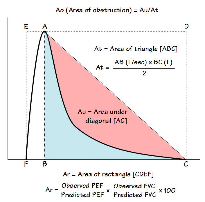
The flow-volume loop is analyzed primarily to determine what the authors call the Area of Obstruction (Ao). To do this, a diagonal line is drawn from peak flow to the end of exhalation. The area that exists between the actual flow-volume loop contour and this diagonal line is defined as the area under the diagonal (Au). The area of Au is then compared to the area of a triangle (At) defined by the peak flow, the exhaled volume at the time of the peak flow, and the end of exhalation. The area of obstruction, which is actually a ratio, is then calculated as:

The more the flow-volume loop curve bows inwards from the diagonal (often described as coving, scooping, or being concave) the closer Ao comes towards 1. When the flow-volume curve is flatter, Ao comes closer to 0. In a sense, Ao describes how concave a flow-volume loop is without actually defining the shape of the contour.

Lee et al also determined what they called the area of the rectangle (Ar, which is basically defined as the percent predicted Peak Flow times the percent predicted FVC), and then other additional parameters, which included Ao/Ar, Ao/PEF and Ao/FVC. From their study population they compared these parameters as well as more routine PFT values such as FEV1, FEV1/FVC ratio and PEF with the RV/TLC (which they considered a marker of hyperinflation) and 6-minute walk distance (6MWD). Statistical analysis showed that all Ao values (Ao, Ao/Ar, Ao/PEF, Ao/FVC) correlated highly with RV/TLC and that Ao/Ar and Ao/PEF correlated better with 6MWD than did FEV1 or the FEV1/FVC ratio.

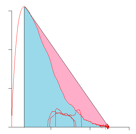
This technique is highly limited both by the observed PEF and by the need for the expiratory curve to be concave as well as the assumption that a diagonal drawn between the PEF and end-of-exhalation describes the ideal expiratory flow rate. Although Ao does to some extent describe the concavity of a loop, this does not necessarily translate well into the degree of obstruction. As an example the following loop has an Ao somewhere around 0.75:

But the results for this loop are quit normal:

	Observed:	%Predicted:	Predicted:
FVC:	4.98	106%	4.69
FEV1:	3.74	105%	3.57
FEV1/FVC:	75	99%	76
PEF:	12.44	136%	9.17

This loop has an Ao around 0.65:

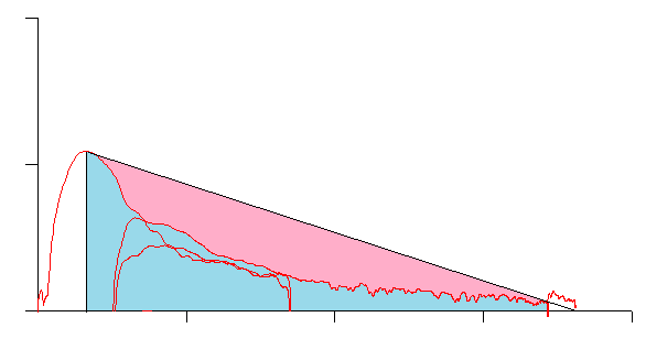
but is from an individual with very severe airway obstruction:

	Observed:	%Predicted:	Predicted:
FVC:	1.81	57%	3.21
FEV1:	0.61	25%	2.43
FEV1/FVC:	33	44%	76
PEF:	1.09	19%	5.88

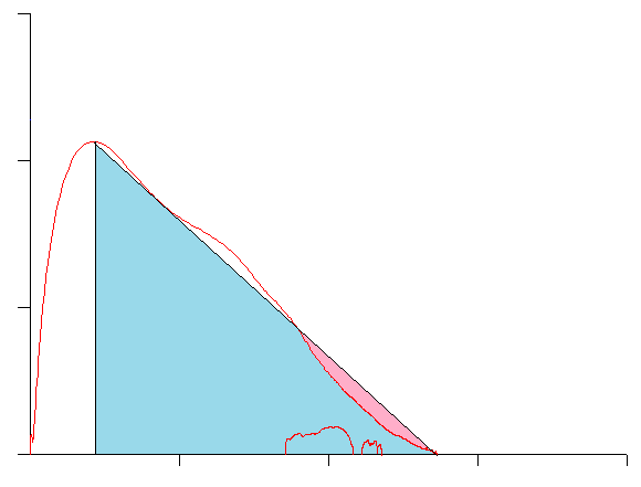
And this approach does not work well with any loops that are convex rather than concave:

For these reasons I suspect that if Lee et al’s study population was broader and contained more subjects with both normal and restrictive lung function rather than just those with COPD, the correlation between Ao, RV/TLC and 6MWD would likely be a lot less statistically significant.

One final issue with Lee et al’s approach is that I never understood the clinical relevance of Ar (the area of the rectangle). Since this area the product of height (peak flow) and width (FVC volume), the area of two very different flow volume loops (think restriction and obstruction) could be very similar. The purpose of Ar and how it was supposed to improve the relevance of Ao (if it did) were not explained.

Kapp et al took a somewhat simpler approach and measured the angle between lines drawn from the MEF@50% to an imaginary point described by the TLC and PEF, and to the end-of-exhalation. This angle (B) can be derived by straightforward geometrical calculations using PEF, MEF@50% and FVC. One advantage of Kapp et al’s approach over Lee et al’s is that it can describe both concave and convex contours (although interestingly Kapp et al used the terms concave and convex oppositely to the current use of these terms which in turn means that not only have the words that have been used to describe flow-volume loops evolved, they have never really been standarized).

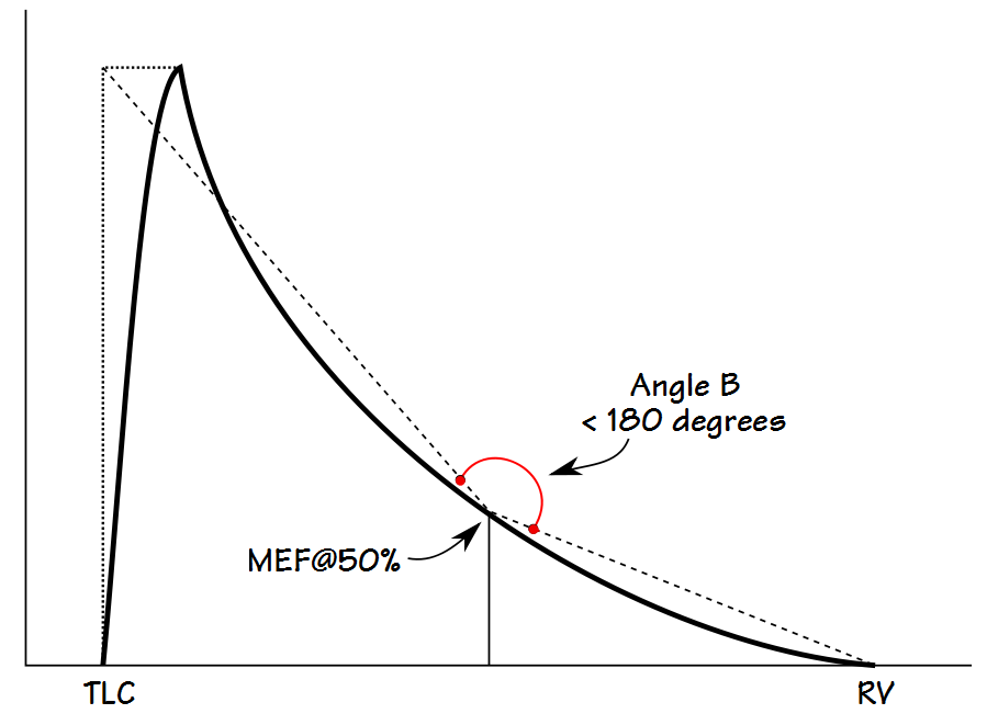
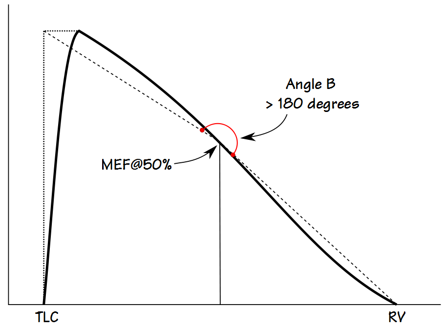
An angle less than 180 degrees indicates a concave expiratory contour and one that is greater than 180 degrees a convex contour. Kapp et all showed that the angle was lower in males than females, and that it decreased with age and with an increase in smoking pack-years. They also categorized the angles associated with different lung diseases, however the overlap between different classifications was significant and so the usefulness of angle B as a discriminating factor is limited.

The weakness of Kapp et al’s approach is that it solely based on an angle that occurs at MEF@50%. In particular, as airway obstruction becomes more severe there is a point at which an inflection point (an abrupt change in expiratory flow rate) appears in the flow-volume loop.

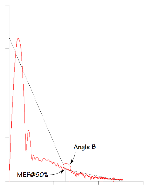
Kapp et al’s Angle B is not able differentiate between the presence or absence of this inflection point. I can also see that Angle B would likely be inaccurate when peak flow is low or delayed, or when expiration terminates early.

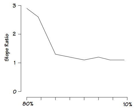
Mead’s approach is probably the most sophisticated since it measures what he termed the slope ratio at intervals throughout exhalation. The slope ratios consist of a comparison of the slope of a line immediately tangent to the flow-volume loop with a chord line drawn from the end-of-exhalation.

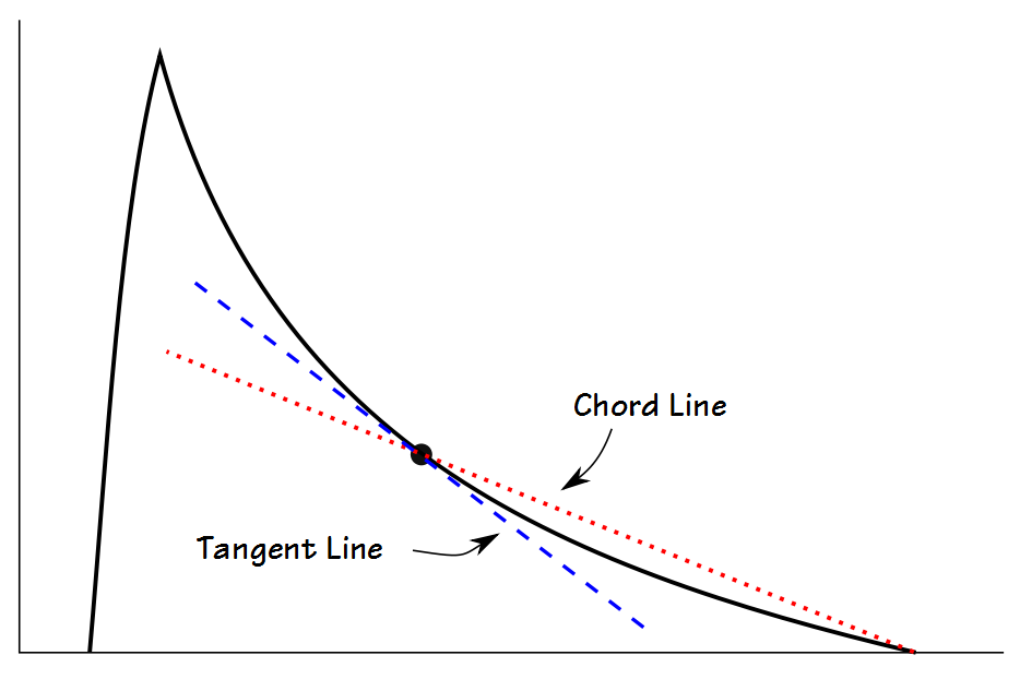
The measurement is then performed at 10% intervals from 80% and 10% of the FVC.

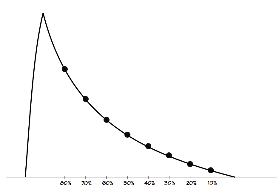
A slope ratio of 1 would indicate a that expiratory flow is straight line between peak flow and the end-of-exhalation. Slope ratios above 1 indicate a concave contour and the degree of concavity increases as the slope ratio grows higher. Slope ratios below 1 indicate a convex contour and the degree of convexity increases as the slope ratio gets closer to 0.

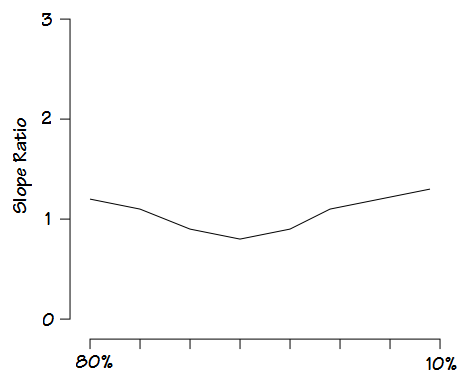
A flow-volume loop likes this:

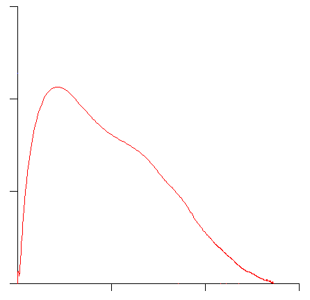
would generate a slope ratio graph something like this:

One like this:

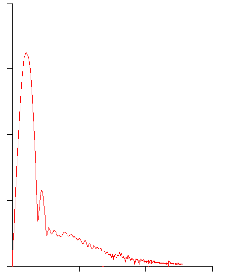
would generate a graph something like this:

Mead was able to show that there were relatively distinct patterns for asthma, chronic bronchitis and emphysema. He was also able to show the distinct changes that occur in asthmatics during exercise-induced bronchoconstriction and post-bronchodilator.

Although Mead’s approach provides more information than the other techniques, I am hard pressed to say that it actually provides more information than can be obtained from the original flow-volume loop. Similarly, although Lee et al and Kapp et al developed methods for quantifying the degree of concavity (and for Kapp et al the degree of convexity as well) of a flow-volume loop, a significant failing (at least from my point of view) in all three techniques is their inability to detect the presence (or absence) of the inflection point that is often seen in severe airways obstruction.

Although I found these different analytical techniques to be interesting, and they have certainly given me something to think about when categorizing flow-volume loop shapes, it is not surprising that graphical analysis of flow-volume loops has shown little or no practical value in the routine interpretation of spirometry results. All of these techniques are entirely dependent on high quality and repeatable spirometry efforts. Any attempt to analyze spirometry efforts with short exhalation times, suboptimal patient effort or poor reproducibility will produce inconsistent and possibly misleading results. In addition, some of the distinctly diagnostic flow-volume loop contours (in particular those with expiratory or inspiratory plateaus) are not recognizable by any of these techniques.

Since Mead’s slope ratio is generated by comparison to a chord line originating from the end-of-exhalation its results are not particularly dependent on peak flow. Both Lee et al and Kapp et al’s approaches however, are highly dependent on peak flow. To some extent this is a problem because ATS/ERS guidelines on the selection of spirometry efforts does not consider PEF at all but are instead only concerned with the highest combined FVC and FEV1.

The most significant problem with any graphical analysis of a flow-volume loop is that all techniques to one degree or another are focused on the concavity (or convexity) the expiratory curve and these factors by themselves do not necessarily differentiate between the presence, absence or degree of airway obstruction. Context is also important. A flow-volume loop that is normal for a 70-year old would likely be considered abnormal for a 20-year old.

I would be interested in a computer algorithm that was able to categorize the shapes of flow-volume loops because this could potentially aid the interpretation of spirometry results in clinics and physician offices. At the moment however, not only is there no standardized terminology, even human categorization is inconsistent. This is partly because there are no really agreed-upon conventions for describing flow-volume loops but it’s also because experience and the ability to judge the quality of a spirometry effort are critical to knowing whether the loop contour is actually diagnostic or just an artifact of a suboptimal test effort, and it is these aspects of the assessment process that are the most difficult to quantify (and to teach).

References:

Kapp MC, Schachter EN, Beck GJ, Maunder LR, Witek TJ. The shape of maximum expiratory flow volume curve. Chest 1988; 94: 799-806.

Lee J, Lee C-T, Lee JH, Cho YJ, Park JS, Oh Y-M, Lee S-D, Yoo HI. Graphic analysis of flow-volume curves: a pilot study. BMC Pulmonary Medicine 2016 16: 18.

Mead J. Analysis of the configuration of maximum expiratory flow-volume curves. J Appl Physiol 1978; 44(2): 156-165.

PFT Blog by Richard Johnston is licensed under a Creative Commons Attribution-NonCommercial 4.0 International License